
How To Establish Sample Sizes For Process Validation Using Variable Sampling Plans
By Mark Durivage, Quality Systems Compliance LLC
The first article in this series, Risk-Based Approaches To Establishing Sample Sizes For Process Validation (June 2016),  provided and established the relationship between risk and sample size. This article will demonstrate the use of variable sampling plans to establish sample sizes for process validation.
Variables sampling was officially introduced in June 1957 by means of MIL-STD-414 Sampling Procedures and Tables for Inspection by Variables for Percent Nonconforming. This standard was officially cancelled in February 1999 and was replaced by ANSI/ASQ Z1.9 Sampling Procedures and Tables for Inspection by Variables for Percent Nonconforming.
I would like to suggest that variable sampling plans should be utilized whenever possible, for two reasons. First, variables data will yield much more information than a comparable sample using attribute data. Second, with fewer samples, associated costs of inspection, measurement, and testing can be substantially reduced.
It should also be noted that a simple random sample is meant to be an unbiased representation of a group. A sampling error can occur with a simple random sample if the sample doesn't end up accurately reflecting the population it is supposed to represent. In other words, each piece that is to be inspected, measured, or tested must have the same chance of being selected and be representative of the batch or lot.
Before we begin, we must establish our definitions of risk and their acceptable quality limit (AQL), the level of quality that will be accepted 95% of the time. These definitions can and should vary based upon organizational needs. A good method for determining risk level is failure modes and effects analysis (FMEA). FMEA (design, process, user) is a systematic group of activities designed to recognize, document, and evaluate the potential failure of a product or process and its effects. FMEA uses a risk priority number (RPN), which is comprised of frequency, detection, and severity. The higher the RPN, the higher the risk; however, a high severity in conjunction of low probability of occurrence and high probability of detection may still necessitate the appropriate controls for high risk. Table 1 depicts an example FMEA with the associated risk levels. Once the risk level has been determined (low, medium, high), the appropriate AQL can be selected using Table 3. Figure 1 depicts the linkage between FMEA, risk, and AQL.
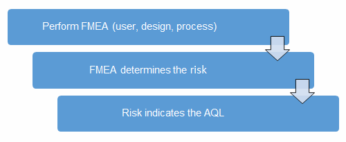
Figure 1: Risk process for determining the appropriate AQL
Table 1: Example FMEA
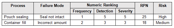
Table 2 shows an example of risk level definitions with accompanying defect classifications. These definitions can and will vary based upon the products produced and their intended and unintended uses.
Table 2: Example of Risk Level Definitions
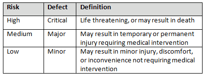
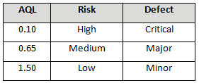
Table 3 depicts example AQLs based upon risk. Different AQLs can and should be utilized based upon the organization’s risk acceptance determination threshold, industry practice, guidance documents, and regulatory requirements. A note of caution when using this method: Lot sizes used for validation activities should be consistent with the lot sizes anticipated for production.
Table 3: Example AQL Based Upon Risk Acceptance
Variable Sampling Plans
When using variable sampling plans, there is an assumption and expectation that the data is normally distributed. There are many ways to determine if data is normally distributed, including computer programs and spreadsheets. However, for small samples (15 or fewer), normal probability plots can be used to assess normality.
Normal probability plots can be constructed to look for linearity when using one variable, providing a visual way to determine if a distribution is approximately normal. If the distribution is close to normal, the plotted points will lie close to a line. Normal probability plots are constructed by doing the following:
- Arrange the data from smallest to largest.
- Determine the percentile of each data value.
- From these percentiles, do normal calculations to determine their corresponding z-scores.
- Plot each z-score against its corresponding data value.
- Perform a graphical review of the normal probability plot for the data points to verify if they generally fall on the line of best fit — sometimes referred to as the “pencil” test. If the data is not normally distributed, it is best to use an alternative method.
(For an example of how to create and analyze normal probability plots, refer to Chapter 4 of Practical Engineering, Process, and Reliability Statistics, ASQ Quality Press, 2014.)
Variable sampling plans can be used for one-sided or two-sided specifications, depending on whether the specification requires a minimum or maximum value or has an allowable range. However, it is generally best practice to use one-sided variable sampling plans — this method will provide a more conservative approach, because the risk is placed on one side rather than being split. If the specification is bilateral, use the specification that is closest to the sample mean, which is calculated from the initial sample. Using one-sided is like calculating the process capability index (Cpk).
Single-Sided Specification Example
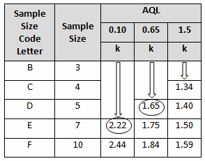
A pouch-sealing operation is considered high risk according the FMEA in Table 1. High risk requires an AQL of 0.10 as shown in Table 3. The specified lot size is 25. From Table 4, a high-risk level with a lot size of 25 yields E for the sample letter code. Using Table 5, an AQL of 0.10 with a sample letter code of E requires seven samples using the critical k value of 2.22.
Table 4: Sample Size Code Letters (Table A-2 Partial)
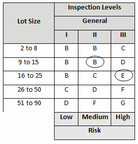
Table 5: Standard Deviation Method Master Table for Normal and Tightened Inspection for Plans Based on Variability Unknown (Single Specification Limit — Form 1) (Table B-1 partial)
The seven samples were found to be normally distributed, with a mean of 3.3 lbs. and sigma of 0.29. The pouch-sealing process specification requires a minimum pull strength of 2.5 lbs.
Note: A minimum of three passing lots would be necessary to make the claim that the validation has met the acceptance criteria and therefore passed.
For a single-sided upper specification:
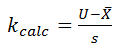
For a single-sided lower specification:
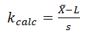
Where:
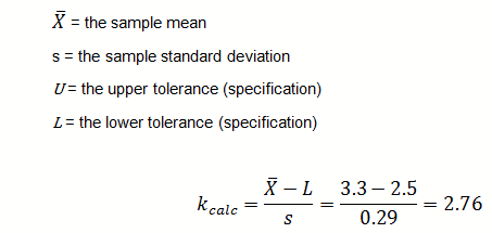
The calculated k value is 2.76.
Since the calculated k value (2.76) is greater than k critical (2.22) the first lot has passed.
Double-Sided Specification Example
A double-sided specification is much like calculating the process capability, or Cpk. The process average is subtracted from the upper specification and subtracted from the lower specification.
A filling operation is considered medium risk according the FMEA in Table 1. Medium risk requires an AQL of 0.65 as shown in Table 3. The specified lot size is 15. From Table 4 a medium risk level with a lot size of 15 yields B for the sample letter code. Using Table 5, an AQL of 0.65 with a sample letter code of B requires five samples using the critical k value of 1.65.
The five samples were found to be normally distributed, with a mean of 996 g and sigma of 4.3. The filling process specification is 1000 g ±10 g.
Note: A minimum of three passing lots would be necessary to make the claim that the validation has met the acceptance criteria and therefore passed.
For the upper specification:
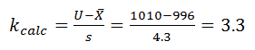
Since the calculated k value (3.3) is greater than k critical (1.65), the upper-sided specification for the first lot has passed.
For the lower specification:
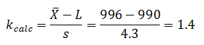
Since the calculated k value (1.4) is less than k critical (1.65), the lower-sided specification for the first lot has failed.
This process has already failed to meet the predefined criteria for the validation. The first thing to try would be to center the process and repeat the validation.
Choosing The Right Technique For Your Process
I prefer to use the single-sided method even with double-sided specifications, to account for an off-center process (same principle as Cpk). Remember, the criteria used should be based upon risk and should be documented and proceduralized. When a validation fails, there are three distinct options available:
- Center the process
- Reduce the variation
- Change the specification (tolerance)
I want to reinforce that different AQLs and risk levels should be utilized based upon an organization’s risk acceptance determination threshold, industry practice, guidance documents, and regulatory requirements. Also realize that the smaller the AQL, the more inspection, measuring, and testing must be performed. Conversely, the larger the AQL, the less inspection, measuring, and testing are required.
This article series has introduced several different methods for establishing sample sizes for process validation. Previous articles in the series including:
- Risk-Based Approaches To Establishing Sample Sizes For Process Validation
- How To Establish Sample Sizes For Process Validation Using The Success-Run Theorem
- How To Use Reliability-Based Life Testing Sampling For Process Validation
- How To Establish Sample Sizes For Process Validation Using C=0 Sampling Plans
- How To Establish Sample Sizes For Process Validation Using Statistical Tolerance Intervals
References:
- ANSI/ASQ Z1.9-2008: Sampling Procedures and Tables for Inspection by Variables for Percent Nonconforming.
- Durivage, M.A., Practical Engineering, Process, and Reliability Statistics, ASQ Quality Press, Milwaukee, 2014.
- Durivage, M.A. and Mehta B., Practical Process Validation, ASQ Quality Press, Milwaukee, 2016.
- Durivage, M.A., Risk-Based Approaches To Establishing Sample Sizes For Process Validation, Life Science Connect, 2016.
About the Author
 Mark Allen Durivage is the managing principal consultant at Quality Systems Compliance LLC and the author of several quality-related books. He earned a B.A.S. in computer aided machining from Siena Heights University and an M.S. in quality management from Eastern Michigan University. Durivage is an ASQ Fellow and holds several ASQ certifications including CQM/OE, CRE, CQE, CQA, CHA, CBA, CPGP, and CSSBB. He also is a Certified Tissue Bank Specialist (CTBS) and holds a Global Regulatory Affairs Certification (RAC). Durivage resides in Lambertville, Michigan. Please feel free to email him at mark.durivage@qscompliance.com with any questions or comments, or connect with him on LinkedIn.