Recovery Studies: Common Issues & Using Statistical Tools To Understand The Data

Part of the Cleaning Validation for the 21st Century series

This article is the first in a series of articles that will explore some of the typical issues that may be encountered during recovery studies and show how the use of statistical tools for assessing the recovery data can provide greater insight into the results and enable data-driven decisions concerning recovery studies. In this installment, we will look at three case studies:

1. Case Study No. 1 will examine how to establish a relationship between the level of compound spiked and the percent recovery through regression analysis. It will also show how regression analysis can be used to provide an indication of how the recovery method works at higher or lower concentrations than those examined in the study.
2. Case Study No. 2 will examine how the 2-sample t-Test might be used to evaluate changes to a swab method to see if the differences in recovery results are significant.
3. Case Study No. 3 will examine how the 2-sample t-Test might be used to evaluate differences in recovery results between two analysts performing swab sampling.

Background

Recovery studies have been an expectation in the GMP world for many years. As far back as 1993, in its guide for inspections on cleaning validation,¹ the FDA stated that:

“The firm should challenge the analytical method in combination with the sampling method(s) used to show that contaminants can be recovered from the equipment surface and at what level, i.e. 50% recovery, 90%, etc. This is necessary before any conclusions can be made based on the sample results. A negative test may also be the result of poor sampling technique... Therefore, early in the validation program, it is important to assure that the sampling medium and solvent (used for extraction from the medium) are satisfactory and can be readily used.’’

It is important to stop and consider what is implied by "early in the validation program": Recovery studies should not be done after sampling has already taken place, but before.

Within a few years, the content of the FDA's guide was adopted almost verbatim in guidelines issued by most regulatory agencies and industry organizations (e.g., EMA, Health Canada, APIC, WHO, etc.). While most of these regulatory guidelines have been updated in recent years, the expectations around recovery studies have remained fairly constant, although in modified form. For example, Annex 15, EudraLex Volume 4, Section 10.12 states more briefly:²

‘’Sampling  should  be  carried  out  by  swabbing  and/or  rinsing  or  by  other means  depending  on  the  production  equipment.  The sampling materials and method should not influence the result. Recovery should be shown to be possible from all product  contact  materials  sampled  in  the  equipment  with  all  the  sampling methods used.’’

Qualifying the recovery of residues, which involves the combination of a sampling procedure with an analytical method, is clearly a regulatory expectation - not only from an analytical perspective but it is also necessary in order to properly train and qualify sampling personnel.^{3, 4, 5}  It is important to understand at this point that recovery studies are concerned with the evaluation of a sampling procedure and not with the analytical method.

One of the issues around recovery studies is what the acceptance criteria should be for the level of recovery. Unfortunately, there is no clear guidance on this. Many people have misread the FDA's statement above to mean that 50 percent is the minimum level acceptable. That is not what the FDA stated.

What has made this issue more confusing is that the various current industry and regulatory guidelines suggest several acceptance criteria for acceptable recovery factors. The Parenteral Drug Association (PDA) suggests that 70 percent is exceptional and 50 percent is adequate.⁴ WHO suggests 80 percent is considered good, >50 percent reasonable, and <50 percent questionable.⁵ APIC suggests 90 percent for exceptional, 50 percent for adequate, and below 50 percent should be omitted.⁶ Literature suggests that operators participating in sampling activities target a recovery of at least 70 percent, with a maximum RSD of 15 percent.⁷

However, in some cases, it may be difficult to obtain a recovery of 70 percent. A recent article advises against discarding such recovery results, even below 50 percent.⁸ A major point of this article is that, while efforts for improving the recovery should be undertaken, the decision on how to handle the results should be in all cases data-driven.⁸

So, while swab and rinse recovery studies have become commonplace at most companies for many years now, there has been poor consensus on what an acceptable recovery should be.

Making this situation worse, there have been many misconceptions spread throughout the industry concerning recovery studies.⁸ There have been claims (unsupported by data) that recoveries decrease as the spike level increases by using analogies to shoveling snow⁹ and even suggesting that because of this, only one spike level should be determined, rather than several levels.^{9, 10} Subsequent to these articles, a published study presented data that contradicted these claims.¹¹ How these data were obtained was questioned, and an analysis of these data with other publications were found to be equivocal.¹² Despite this finding, this author continues to assert that only one spike level is sufficient.¹³

There is also the assertion that the amount spiked on coupons should be at the swab acceptance limit based on the MAC (maximum allowable carryover) calculation.^{7, 9, 13, 14} As swab acceptance limits based on the MAC can vary widely due to differences in the calculation parameters (therapeutic dose, total surface area, etc.), spiking at these levels may have more of an impact on the recovery than the swabbing technique used. In one case, the spike level based on the MAC calculation may be low and recovery is high, while for another, the spike level may be high and the recovery is low.

This article will examine the data from three swab recovery studies for three different APIs that have some interesting results to review considering the above discussion. These studies were almost identical in their execution but were conducted with slight differences.

Case Study Parameters

For all three studies, solutions of three active pharmaceutical ingredients (APIs) – "H," "L," and "P" – were prepared at concentrations ranging from 50 to 150 ppm. All studies used the following parameters with some slight differences. These differences and why they occurred will be discussed in each case study.

Coupon spiking was performed as follows:

1. A 1 mL volume of each solution was spiked onto one 10 x 10 cm² 316 L stainless steel coupon surface.
2. The 1 mL spike was distributed in five droplets of 200 μl each onto the coupon surface.
3. The five droplets were distributed on the coupon by spiking near the four corners and the center of each coupon.
4. All coupons were allowed to dry before being swabbed.

Swabbing was performed using the following technique:

1. All swabs were dipped in suitable solvent and slightly shaken for excess solvent to be removed.
2. The coupon surface was sampled with horizontal (or vertical) continuous movements.
3. The swab was flipped and swabbing was repeated in the opposite or perpendicular direction with continuous movements.
4. The surface was checked for spots: if spots were still present on the coupon (this might happen if a solvent with high surface tension, like methanol,¹⁵ was used in the solution preparation), the analyst swabbed the surface using the tip of the swab.

Analytical method: HPLC was the method of choice for these studies, as it is substance specific. For HPLC, the solvent used in standard solutions preparation, as well as the solvent used for wetting the swabs prior to sampling, is important.  All swabs were immersed in 2 mL of the solvent used for the solutions preparation and analyzed by HPLC. While HPLC provides the advantage of high specificity for detection of the substance under evaluation, nonspecific methods, such as total organic carbon (TOC), can also provide effective swab recovery methods.¹⁶

Case  Study  No.  1

For Case Study No. 1, the API was "H" and the solvent used for spiking and swabbing was ethanol (EtOH). The results are shown in Table 1.

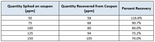
Table 1: Recovery of active pharmaceutical ingredient ‘’H’’ in ethanol. Results are expressed in parts per million (ppm).

These data were subjected to a linear regression analysis using Minitab (Figure 1).

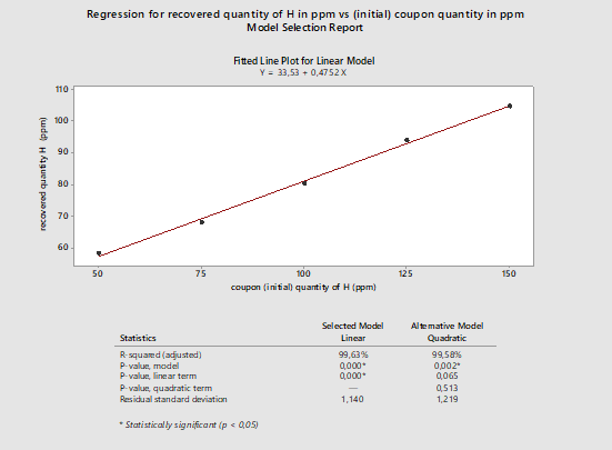
Figure 1: Regression analysis for active pharmaceutical ingredient H recovery. This data is based on a single analyst (Analyst A). The data has been plotted in ppm of recovered quantity versus spiked quantity in ppm. (Note: the high recovery at 50 ppm was investigated, and an error in the 50-ppm solution preparation was confirmed.)

The graph in Figure 1 shows an apparently linear response with a model of Y = 33.53 + 0.4752X. On first examination, there appears to be a strong correlation between the spiked amount and the recovered amount. If we analyze the linear regression model, we see that the Y-intercept is 33.53, which means that for a standard concentration of 0 ppm we should expect to recover at least 33.53 ppm, which of course should not be possible. It is recommended that a zero point (coupon blank) should be run with every recovery study.

We can also see that the slope is 0.4752, which means that for 100 ppm of standard quantity, we should expect a recovery of approximately 48 ppm, or about 50 percent recovery. At higher concentrations, the model provides recovery results closer to the actual data. For example, for a spiked quantity of 100 ppm, based on the model the recovered quantity is approximately 81 ppm. This is quite close to the result we see in Table 1: For the spiked quantity of 100 ppm, the recovered quantity was 80 ppm.

One major issue in general with spiking at high levels such as these is that they are not representative of the levels that will be encountered during actual cleaning qualification studies. If the cleaning process has been appropriately developed,¹⁷ then any process residues should be at or below the Detection Limits (DL) or Quantitation Limits (QL) of the method. Poor recoveries at these high levels should not be translated into poor recoveries at levels near the DL or QL. Most often, recoveries at levels near the DL or QL are almost 100 percent. Therefore, recovery studies should be performed at multiples of the DL/QL and not at the levels of the Acceptable Residue Level (which, as noted in the background discussion above, may be very high) to obtain the true recovery levels and to cover the actual range of expected results.

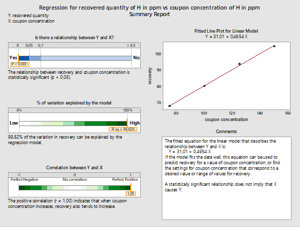
Figure 2: Summary report for the linear model fitted using Minitab 18 for recovered versus initial coupon concentration of active pharmaceutical ingredient H. (Note: 50 ppm recovery data were removed from this analysis.)

In regression analysis, an important measure is the p-value, which represents the margin of error we are willing to accept, if we accept that the respective model represents the data. Usually, the accepted Type I error is set at 5 percent, or a level of significance of 0.05 (i.e., p-value ≤0.05). If the p-value is above 0.05, we might reject the model. The lower the p-value, the greater the confidence we have in accepting the model based on our data.

In Figure 2 we can see the summary report for the linear model. The p-value is below 0.001, which is well below 0.05; therefore, there is a vey strong probability that this model accurately describes the relationship between recovered and initial coupon concentration.¹⁸

According to ICH_Q2b [19]:

‘’...an analysis of the deviation of the actual data points from the regression line may also be helpful for evaluating linearity’’.

Since it is established that the linear model fits the data, we can proceed with exploring further options provided by Minitab 18. One of them is the prediction report, which provides the predicted values for the recovered versus initial quantities, as well as the 95 percent probability intervals for the recovered quantities, based on the linear model (see Figure 3).

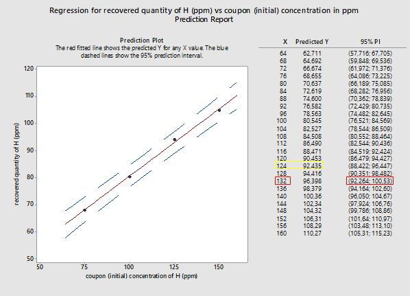
Figure 3: Probability intervals (95%) for recovered quantities versus initial quantities placed on coupons (both in ppm of substance H). X represents the coupon concentration in ppm while Y represents the recovered quantity, also in ppm. (Note: 50 ppm recovery data were removed from this analysis.)

In a recovery study, the spiked or initial coupon concentration (X) is known and, through the analysis, the recovered quantity (Y) becomes known. For a cleaning validation trial, the case is quite the opposite: the residue quantities recovered from equipment (the results of the swabs analysis) are known, while the initial quantity of residues on equipment (residues left on equipment surface at the end of cleaning operations) is unknown.

Here we attempt to use the results of the prediction report for the linear model, as shown in Figure 3, to explore recovery at various concentrations.

For example: A swab result, as part of a cleaning validation sampling session, is 92 ppm (yellow square in Figure 3). This quantity is recovered from equipment. In this case we know that the Y value is 92 ppm and look for the X value. If we use the results given in Figure 3, for an expected recovery of 92 ppm, the X value would be 124 ppm. So, for a recovered from equipment quantity of 92 ppm, we can expect that the actual quantity of residue on the equipment surface at the end of cleaning operations was 124 ppm. The respective values are outlined in yellow in Figure 3.

A more conservative approach would be to consider the swab result as the minimum possible recovered quantity.  In that case, we make the assumption that the recovered quantity is attributed to the lower 95 percent probability interval. Going back to our example, let’s suppose we recover from equipment a swab result of 92 ppm. In Figure 3, we see that the closest 95 percent lowest interval limit to 92 ppm is the lower limit of the interval (92.264; 100.53) (values are outlined in red in Figure 3). For that interval, the respective Y value is 132 ppm. That would be interpreted as: For a recovered from equipment quantity of 92 ppm, we can assume that the actual quantity of residue on equipment surface, at the end of the cleaning operations, would be as high as 132 ppm.

In a recent article, M. Ovais summarizes current literature approaches in selecting a recovery factor.⁸ In this article, it is strongly supported that any decision should be data-driven and that selecting the lowest confidence interval delivers, in most cases, a safer approach than choosing the mean or average recovery. However, in many cases, this approach can be unnecessarily rigid.⁸

Case  Study  No.  2

Case Study No. 2 is an example of how the 2-Sample t-Test analysis can be used to assess the result of changes in the recovery method.

Initially, solutions of concentrations from 50 to 150 ppm of active pharmaceutical ingredient L in 1:1 methanol (MeOH) to 2 percent NaOH in purified water (v/w) were studied for recovery. The swabs were analyzed with HPLC. This method obtained less than ideal results. In an attempt to improve the recovery results, a few alterations to the method parameters were made.

The main differences between the first and the second trial were the following:

• The solvent for solution preparation: the solvent used for the first trial was 1:1 methanol (MeOH) to 2 percent NaOH in purified water (v/w). For the second trial, a more volatile solvent, ethanol, was used. That not only had the advantage of reducing the coupon’s drying time, but it also improved the uniformity of the active ingredient solution over the coupon surface during the spiking process.
• The spiking process for coupons: for the first trial, during the spiking process the solution was deposited in droplets due to the high surface tension of methanol.¹⁵ After evaporation of the solvent, there were visible spots on the surface. For the second trial, ethanol was used. Ethanol spreads rapidly over the coupon surface due to low surface tension. The analysts were instructed not to spike close to the coupon’s edges in order to avoid loss of quantity over the coupon surface.
• Analyst training & sampling instructions: for the second recovery study, the analysts were advised to use more deliberate swabbing movements. They were also instructed to swab the coupon perimeter in order to gather as much residue as possible.⁷

Results for both trials are shown in Table 2:

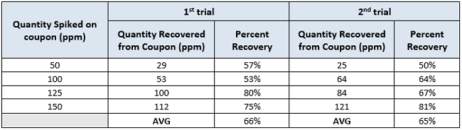
Table 2: Recovery of active pharmaceutical ingredient L for the two recovery trials (in 1:1 MeOH : 2% NaOH in PW for the 1^st and EtOH for the 2^nd recovery trial). Results are expressed in parts per million (ppm).

From a first look we see that the average percent recovery appears to be slightly decreased for the second group of results. Despite the efforts for improvement, the recovery was not improved for the second trial.We would like to explore how statistically significant any difference is between the two groups using the 2-Sample t-Test.

Statistical tests like the 2-Sample t-Test compare the "null hypothesis" - that there is no significant difference between specified populations and that any observed difference is due to experimental error - to an "alternative hypothesis" that there is some difference. Here the 2-Sample t-Test compares the means of two groups of data with each other. In this 2-Sample t-Test we are assessing whether the differences between the means of the two studies are statistically significant.^{20, 21}

There are three options when performing the 2-Sample t-Test hypothesis testing for the sample means: equal to each other, less than, or greater than. Here we choose to test whether the results of the first trial (Recovery_1) are greater than the results of the second trial (Recovery_2). This analysis was performed with Minitab 18. In Figure 4 we see the Summary Report by Minitab 18 summarizing the outcome of the evaluation.

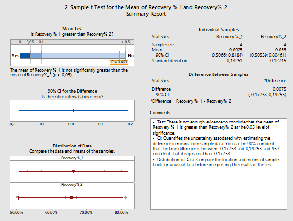
Figure 4: 2-Sample t-Test report for recovery % of the 1^st versus the 2^nd trial: Assessing the effect of changes in recovery factors using the 2-Sample t-Test for first versus second trial. For the second trial, changes in the solvent, the spiking process, and the sampling instructions were performed.  Though the mean of the second run is lower and there is less variability as the standard deviation is lower, no significant statistical difference was found. (Minitab 18 uses Welch method since the samples belong to different populations and have unequal variances.)

In this case our alternative hypothesis could also be stated as: ‘’Is the mean recovery of results of the first trial higher than the results of the second trial?’’. The confidence level for the hypothesis tested here is 95 percent, which would mean accepting a sampling or experimental error probability of 5 percent or 0.05. The probability value for the hypothesis test is higher than 0.05 (p-value = 0.469); therefore, we can assume that the hypothesis should most likely be rejected in favor of the null hypothesis (no difference).²⁰ Any differences between the two methods could be attributed to chance or error. This means if we were to repeat both methods and compare the results, there is a possibility that the first trial might provide a lower recovery percentage than the second trial.

Minitab 18 also provides the option of testing the power of the test based on our sample size. In Figure 4 we see the diagnostic report provided by Minitab for the 2-Sample t-Test of the two sub-groups:

Figure 5: Diagnostic report for the 2-Sample t-Test results for 1st vs 2nd trial for active pharmaceutical ingredient L.

In Figure 5 we see that the smaller the difference between the two groups we want to detect, the smaller the possibility of detecting the true difference between the two groups. If we narrow the difference we want to detect, our estimation has greater uncertainty. In that case, we will also need a larger number of samples.

Summarizing the outcome of Case Study No. 2, we see that though an attempt was made to improve the recovery method, it did not deliver significant results. There is an inherent variability in recovery methods, and results do not always meet expectations.⁸

In this example, since we saw that there is no statistical difference between the two methods, our choice would be based on certain factors. In the second method, we used ethanol, a more volatile solvent that required less preparation time compared to the solvent in the first method (methanol in purified water). In addition, ethanol is relatively less toxic than methanol: it is categorized as Class 3 solvent (solvent with low toxicity potential), while ethanol is categorized as Class 2 (solvent to be limited) by ICH_Q3C.²² In the end, the second method would be more likely to be selected, but the first method would perform just as well in terms of recovery.

Case Study  No. 3

The recovery study results can serve as documented evidence of personnel training and qualification. Sampling results by operators who follow the same sampling instructions should not deviate significantly, or at least they may deviate within specific limits. Analyst training and experience play an important part in recovery studies. Training of operators in sampling is a means to reduce subjectivity in terms of the sampling technique and eliminate differences between different operators.^{3, 23, 24} Therefore, training of operators in the sampling method is essential. Case Study No. 3 will show how differences between operators performing the same recovery study can be demonstrated.

Two analysts (Analyst A and Analyst B) participated in a recovery study of an active ingredient ‘’P.’’ Analyst A was more experienced in sampling for cleaning validation purposes compared to Analyst B. Analyst B was still being trained at the time of the study and participated for the first time in the qualification of swab recovery.

For this study, two sets of five coupons were used. The solvent solution used throughout the study for the API was ethanol.

For each analyst there is a set of five recoveries available, for coupon concentrations of 50, 75, 100, 125, and 150 ppm applied on a surface of 10 x 10 cm².

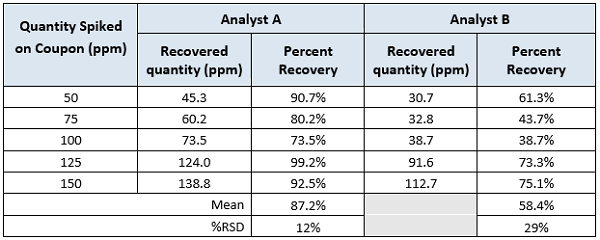
Table 3: Recovery of active pharmaceutical ingredient ‘’P’’ in ethanol. Results are expressed in parts per million (ppm).

As in Case Study 2, a quick examination of these data would conclude that there is a difference in the results for the two analysts. As mentioned in the background discussion, one author set the minimum acceptance value for an analyst at a minimum of 70 percent and the maximum RSD at 15 percent.⁷ Both analysts would pass the minimum recovery criteria provided by most regulatory guidance documents.^4,5,6 Analyst A would pass the maximum variation provided  by literature,⁷ but Analyst B would not. Obviously, the variation for the recovery results between analysts would be greater, for example, 20 or 25 percent. The question is how much variation is acceptable and how can we determine what the maximum should be? These data can be evaluated using 2-Sample t-Tests looking for differences in the means to provide insight into these questions.

In Figure 6, we evaluate the difference in recoveries between two analysts (recovery 1 for Analyst A, recovery 2 for Analyst B) through 2--Sample t-Test for the means using Minitab 18. The hypothesis tested here is: ‘’Is the mean recovery of Analyst A always higher than the mean of Analyst B?’’

The hypothesis testing has a clause: what value of difference between the two means would be considered significant? Here the difference is set at 5 percent (depending on internal company procedures, the difference could be set at a more or less stringent level). Results are presented in Figure 6.

Figure 6: Hypothesis testing for recovery data from Analysts A (recovery_1) and B (recovery_2).

The confidence level for the hypothesis tested here is 95 percent, which would mean accepting an error probability of 5 percent, or 0.05.  The probability value for the hypothesis tested is lower than 0.05; in Figure 6 we see that the p-value is 0.008. Therefore, we can assume that the null hypothesis can be safely rejected in favor of the alternative hypothesis.

In Figure 6 we also see the individual 90 percent confidence intervals for each analyst as well as the confidence intervals for the difference between the means. The difference between the two analysts could range from 11.8 to 45.8 percent. If we are to accept a difference in the recovery data obtained by different analysts then (again depending on internal company procedures) the difference for the 2-Sample t-Test can be set at 1 percent, 2 percent, or 5 percent.

It is important to note that the difference between the recoveries of the two analysts is not to be confused with the margin of error we set for the hypothesis testing above. The first refers to the recovery factor while the second to the probability of the hypothesis scenario being true.

Figure 7: The power of the hypothesis tested here depends strongly on the sample, which would be the number of data available.²⁵

Minitab provides a diagnostic report for the evaluation of the two data sets, which we see in Figure 7. The observed difference between the two means is 28.8 percent. With the available data, there is only a 12.9 percent chance of making sure we detect a minimum difference of 5 percent. The broader the difference we are willing to detect (for example 10 percent, 12 percent, etc.), the less data would be needed for it to be detected. If we narrow the difference, many more samples would be required (133 for 90 percent power).

Analysts A and B participated in the study for personnel qualification for sampling manufacturing equipment, as part of the cleaning validation studies. Considering the variability of the sampling procedures, assuming that Analyst A would always sample better than Analyst B seems a logical conclusion. So, this is where the hypothesis testing (e.g., a 2-Sample t-Test) could provide better insight than making an assumption based on simply comparing the means of the recovery results.

Analyst training and experience play an important part in recovery studies.^{3, 23, 24} Training of operators in sampling is a means to reduce variability of the sampling technique and eliminate differences between different operators.^{3, 24} Although some publications have suggested that the effect of analyst contribution is minor and that effectiveness of the method lies mostly in the choices related to the analytical method,⁷ the authors believe that training of personnel in the swabbing technique plays an important part in the process. In many cases, the variation from swab sampling exceeds any variation from the analytical method.

As part of a broader personnel training and qualification program, would it make sense to give Analyst B some extra training and preparation before assigning them as sampling personnel? How much closer to Analyst A should the results of Analyst B get in order to accept that no matter who is assigned to the sampling tasks for cleaning validation, recoveries remain within the defined acceptance criteria? These will need to be decided based on risks identified and internal company policies but will also need to be supported by statistical analysis of the results.

Discussion Of t-Tests

Averaging of the results for recovery studies that involve several levels has been a common practice for many years. As we saw in this article, recovery results can vary widely, so another practice has been to use the lowest recovery value obtained. When calculating averages, the next obvious step is to obtain the standard deviation and then to calculate the %RSD (Relative Standard Deviation).  Since the sample size is also known (n), it is another short step to using one of the several t-Tests available to make comparisons between recovery studies, since these tests use the average, standard deviation, and n.

Before using any t-Test there are some underlying assumptions that should be considered:

• The data being compared should follow a normal distribution.
• The data being compared should have the same variance.
• The data should be sampled independently from the two populations being compared.

Despite these requirements, most of the 2-Sample t-Tests are robust to all but large deviations from these assumptions.²⁶ Also, the t-Test is highly robust to the presence of unequal variances if the sample sizes are equal.²⁷ All the data in the t-Tests in this article passed the Normality Test in Minitab, the data were samples from different populations (recovery studies), and their sample sizes were equal. So, the use of the 2-Sample t-Test can be justified in these case studies.

However, there are some aspects concerning the data that need to be considered. All this recovery data comes from single samples of multiple spike levels, so the data points are not specifically samples of the same group. If replicates had been performed at each level, then each level could be compared within the recovery study and then each level could be compared between the two recovery studies. This would be a more appropriate and exacting comparison. Alternative approaches will be examined in the subsequent articles. Regardless, the 2-Sample t-Test provides a much more useful and insightful tool for evaluating recovery results than simply calculating an average of the recovery data.

These studies examined the use of the 2-Sample t-Test, which is used to test the difference between two population averages to determine whether the averages are equal. Another test, called the paired t-test, is used for before and after observations on the same subjects and is appropriate for the test conditions found in these case studies and would have even greater power and accuracy.

Summary

Although the recovery of sampling and associated analytical methods have been the topic of considerable regulatory scrutiny, there is no clear guidance on how to establish the acceptability of the sampling procedure. There still appears to be much trial and error in the process of obtaining acceptable recovery, establishing acceptance criteria for the results, and the training and qualifying of sampling personnel. In this article, an effort was made to examine evaluation of results, not just in terms of meeting regulatory acceptance criteria, but in a broader perspective.

It should be noted there is value in performing recovery studies over a range of concentrations instead of simple replicates at one concentration.^{9, 10, 12, 13} It should also be understood that spiking at the acceptance limits can easily lead to poor recovery results that are not reflective of the range where actual data should be found. Studies should be performed at multiples of the detection/quantitation limits. As seen from these case studies, a great deal of information can be revealed through regression analysis, hypothesis testing, and exploring confidence intervals that will be completely missed with studies at a single level. Typical misconceptions around recovery studies have been discussed thoroughly in a previous article.⁸ Recovery factors do not always meet the regulatory acceptance criteria. Rather than struggling to fit the data into a narrow perspective, it is much more useful to reveal the actual tendencies.⁸

Statistical analysis provides powerful tools for assessing the data in the process of developing an optimal sampling method.  These tools can provide insight into data tendencies, evaluating changes, and for comparing data. In the decision-making process regarding method finalization and personnel qualification, statistics can provide not only the expected regulatory supportive evidence but also the confidence that any decision is data-driven.

Future articles will expand further on the application of statistical techniques in validating recovery studies for cleaning validation.

Peer Review:

The authors wish to thank Bharat Agrawal; Ralph Basile; Sarra Boujelben; Joel Bercu, Ph.D.; Gabriela Cruz, Ph.D.; Mallory DeGennaro; Kenneth Farrugia; Andreas Flueckiger, M.D.; Igor Gorsky; Robert Kowal; Mariann Neverovitch; Miquel Romero Obon; Osamu Shirokizawa; Siegfried Schmitt, Ph.D.; Ruijin Song; Stephen Spiegelberg, Ph.D.; and Ersa Yuliza for reviewing this article and for providing their insightful comments and helpful suggestions.

References:

1. U.S. Food & Drug Administration ‘’Validation of Cleaning Processes 7/93: Guide to Inspection of Cleaning Processes’’
2. EudraLex Volume 4 EU Guidelines for Good Manufacturing Practice for Medicinal Products for Human and Veterinary Use Annex 15: Qualification and Validation
3. Kalelkar, S., J. Postlewaite, Sampling for Cleaning Validation: Analytical considerations, Cleaning and Cleaning Validation Vol.2, Paul L. Pluta Editor, PDA Bethesda MD, USA, DHI Publishing LLC
4. PDA, Technical Report No. 29 (Revised 2012) - Points to Consider for Cleaning Validation, 2012.
5. World Health Organization, Technical Report Series 937, 40th Report. Annex 4 Supplementary guidelines on good manufacturing practices: validation, Appendix 3 Cleaning Validation
6. Active Pharmaceutical Ingredients Committee, Guidance On Aspects Of Cleaning Validation In Active Pharmaceutical Ingredient Plants, Revision September 2016
7. Forsyth, Richard J. Best Practices for Cleaning Validation Swab Recovery Studies, Sep 02, 2016 Pharmaceutical Technology Volume 40, Issue 9, pg 40–53
8. Ovais, Mohammad, On Cleaning Validation Recovery Studies: Common Misconceptions, Published on IVT Network (http://www.ivtnetwork.com), June 22 2017
9. Destin A. LeBlanc, Spiking Amounts for Sampling Recovery Studies, Memo July 2007, (http://www.cleaningvalidation.com/memos.html)
10.  Destin A. LeBlanc, Revisiting Linearity of Swab Recovery Results Memo July 2009 (http://www.cleaningvalidation.com/memos.html)
11. Pack, Brian W. and Jeffrey D. Hofer "A Risk-Management Approach to Cleaning-Assay Validation" Pharmaceutical Technology  2010 Volume 34, Issue 6
12. Swab Sampling Recovery as a Function of Residue Level, Memo September 2010, (http://www.cleaningvalidation.com/memos.html)
13. Destin A. LeBlanc,  Revisiting Linearity of Recovery Studies September 2013 (http://www.cleaningvalidation.com/memos.html)
14. Richard J. Forsyth, Rethinking Limits in Cleaning Validation: An integrated approach can improve the efficiency of cleaning validation studies, Oct 02, 2015, Pharmaceutical Technology Volume 38, Issue 10
15. Ghahremani H., A. Moradi, J. Abedini-Torghabeh, S.M. Hassani, Measuring surface tension of binary mixtures of water + alcohols from the diffraction pattern of surface ripples, Der Chemica Sinica, 2011, 2(6):212-221, www.pelagiaresearchlibrary.com
16. Walsh, Andrew & Altmann, Thomas & Canhoto, Alfredo & Barle, Ester & G Dolan, David & Flueckiger, Andreas & Gorsky, Igor & Kowal, Robert & Neverovitch, Mariann & Ovais, Mohammad & Shirokizawa, Osamu & Waldron, Kelly. (2018). A Swab Limit-Derived Scale For Assessing The Detectability Of Total Organic Carbon Analysis, Pharmaceutical Online, January 2018
17. ASTM E3106-18 “Standard Guide for Science-Based and Risk-Based Cleaning Process Development and Validation” https://www.astm.org/Standards/E3106.htm.
18. G. Keller, Statistics for Management & Economics, 10^th edition, Chapter 16: Simple Linear Regression & Correlation
19. ICH Harmonised Tripartite Guideline Analytical Method Validation Q2b Current version
20. G. Keller, Statistics for Management & Economics, 10^th edition, Chapter 13: Inference about  comparing two populations
21. http://www.biostathandbook.com/pairedttest.html
22. ICH Harmonised Tripartite Guideline IMPURITIES: GUIDELINE FOR RESIDUAL SOLVENTS Q3C(R5), Current Step 4 version
23. Kundu, Samar K, Guidance to Cleaning Validation in Diagnostics, 2012
24. Raval, Kashyap, A review of Cleaning Validation Sampling Techniques, EUROPEAN JOURNAL OF PHARMACEUTICAL  AND MEDICAL RESEARCH,  ejpmr, 2016,3(7), 202-206
25. http://www.itl.nist.gov/div898/handbook/prc/section1/prc14.htm
26.  Bland, Martin (1995). An Introduction to Medical Statistics. Oxford University Press. p. 168. ISBN 978-0-19-262428-4.
27. Markowski, Carol A.; Markowski, Edward P. (1990). "Conditions for the Effectiveness of a Preliminary Test of Variance". The American Statistician. 44 (4): 322–326.