Calculating Process Capability Of Cleaning Processes With Completely Censored Data

By Andrew Walsh, Miquel Romero Obon, and Ovais Mohammad

Part of the Cleaning Validation For The 21st Century series

Data that are below the detection limit (DL) are known as left-censored data. A previous article¹ discussed how cleaning process capability can be estimated where some of the cleaning sample data are below the DL. Quite often, though, all the results of the cleaning samples (by methods such as HPLC, UV-Vis, etc.) fall below the detection limit. In these cases, the data are completely (100 percent) left-censored data. How can cleaning process capability be calculated in such situations? This article will explore several approaches that can be used to estimate cleaning process capability when 100 percent of the sample data are below the DL.

We have seen how the Maximum Likelihood Estimate (MLE) can estimate a mean and standard deviation from partially censored data and that these parameters can then be used to generate data to replace the left-censored data, allowing process capability to be calculated.¹ But in cases where all of the data are less than the detection limit, there is no actual data to perform an MLE analysis on, generate a "fitted" best distribution, calculate a mean and standard deviation, and then use these parameters to generate the missing data. Can some of the insights from the MLE analysis also be applied to data sets that contain 100 percent left-censored data?

It should be understood that a result of "less than DL" does not mean zero. And, while left-censored data cannot be quantified, it is understood that their "true" values lie somewhere between zero and the DL. So, it is not unreasonable to generate a distribution of data that is all above zero and all below the DL of the method, and then estimate the process capability from this distribution. There are many statistical software packages available (e.g., Minitab, JMP, R, etc.) that can generate a data set of any size and following whatever probability distribution you wish to use. These packages only require that you select the type of distribution you want, enter the parameters needed for that distribution, and enter the number of data points you wish to generate.

As discussed in a previous article,² it is reasonable to assume that the "true" values for data points below the DL would be normally distributed as swab samples are the sums of multiple independent random variables (residue variability, sampling variability, dilution variability, analytical variability, etc.), which, according to the central limit theorem, will tend toward normal distributions.³

Approach Assuming A Normal Distribution

If we decide to generate data from a normal distribution, then we need to provide a mean and a standard deviation. The mean and standard deviation selected must be values that would generate a data set that is above zero but also below the detection limit. As noted above, the number of data points we should generate should equal the number of left-censored data in the data set we are interested in analyzing. That is, if our data set contains 36 data points that are all less than the DL, then we should generate a similar amount of data as those hidden under the DL.

Next, there should be two goals:

1. The data set generated must fit within the boundaries of zero and the DL with no data points exceeding these boundaries.
2. The data set generated should also provide the lowest possible process capability (as a worst case estimate).

Consider a situation where we have 150 swab samples in which all the analytical results are < DL. To estimate the cleaning process capability, we need to generate 150 values that are above zero but below the detection limit. Figure 1 shows a histogram of 150 data points from a normal distribution with a mean of 35 ppb and a standard deviation of 10 ppb generated using the Minitab random number generator.

Figure 1: Histogram of Generated Normal Data with a Mean of 35 and a Standard Deviation of 10. Reference line added to show the detection limit of 50.

While all of the data are above zero, the histogram in Figure 1 clearly shows that a significant number of these data points are above the DL of 50 ppb. If all of the data in the data set you wish to analyze are left-censored, then this simulated data set does not truly represent those data. Either the mean (35 ppb) was set too close to the DL (50 ppb) or the standard deviation (10 ppb) was set too wide (or both) and this allowed some data points to cross the DL. Any values used for the mean and standard deviation should generate a data set that is above zero but also completely below the DL. So, in this example, the simulated data set does not represent the left-censored data set and would result in a process capability result that is worse than it actually is.

We could approach this in a trial-and-error fashion where we try various combinations of means and standard deviations until we find the most appropriate combination, but is there a better way of selecting the mean and standard deviation for these data sets?

Actually, an appropriate selection of the mean and standard deviation can be very easily accomplished by simply setting the mean to the midpoint between zero and the DL and then setting the standard deviation to one-third of the midpoint value. This would approximate a distribution with a process capability of 1.0 or a 3 Sigma process (See reference 4, Calculating Process Capability of Cleaning Processes: A Primer). This will result in a data set that will fit perfectly between the DL and zero and give (probabilistically) the lowest process capability that meets goals 1 and 2 (Figure 2). This approach greatly simplifies the analysis.

Figure 2: Process Capability for Simulated Data with a Mean of 25 and a Standard Deviation of 8.3. The midpoint between 0 and 50 is 25 and one-third of 25 is 8.33. Reference line added to show the detection limit of 50.

Graphical Approach Assuming A Normal Distribution

Another approach that can simplify this analysis for the cleaning validation specialist is to use the graph in Figure 3. Figure 3 shows the Cpu for each pair of mean and standard deviation meeting goals 1 and 2 defined above and also considers the relationship between DL and the acceptance limit. This graph was created using the z distribution formula (centered and standardized Gaussian distribution, a normal distribution with mean=0 and standard deviation=1).

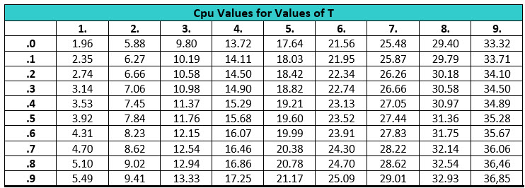
Figure 3: Process Capability Upper (Cpu) vs. How many Times (T) the Acceptance Limit is Higher than DL Worst case for each line is reported in the left boxes. X axis values correspond to the mean value expressed as fraction of DL. Mean values < DL/2 are not shown because any normal distribution with those means would have lower standard deviations than the reported worst case to avoid negative numbers. Values T<1.0 are not reported since these values are not possible (meaning that USL would be lower than DL).

To use the graph above, you start by simply dividing your acceptance limits with your DL (T). For example, for an acceptance limit = 100 ppb and DL = 50 ppb, the T value would be 2. For T= 2.0, the worst Cpu is 5.88. In other words, if all results fall below DL, Cpu=5.88 can be assumed since the real value would be Cpu ≥ 5.88 under the assumption that the data is normally distributed.

Table 1 shows Cpu values from T=1.0 to 9.9 in steps of 0.1. Calculations were made for a number of samples ≥ 30.

Approach Assuming A Non-Normal Distribution

While the argument for using a normal distribution for left-censored data based on the central limit theorem has its merits, it is truly challenging to know exactly which distribution is correct to use. As we noted in our "primer article,"⁴ the statistician George E. P. Box famously said, "all models are wrong; but some are useful." So, distributions other than the normal may be useful for this type of analysis also.

Another argument might also be to consider that the data would not be normally distributed since there is a definite boundary at zero and these data would naturally tend to skew to the right, resulting in a non-normal distribution. This argument has merit as well. There are a large number of distributions that are bounded by zero that could also be used to model these data, but most of them have origins and uses in unrelated fields, such as insurance and wireless communications. One of these distributions is the lognormal distribution, and there have even been some publications over the years arguing that the lognormal distribution is actually more common in nature and the normal distribution should not be assumed as much as it is.⁵ So, the lognormal distribution is worth examining also.

As with the normal distribution analysis above, 150 data points were simulated but using the parameters used for lognormal distributions instead. Unlike the normal distribution, the lognormal distribution belongs to a family of probability distributions that uses parameters other than the mean and standard deviation. These are the "threshold" parameter (which in our case should be zero), a "location" parameter, and a non-negative "scale" parameter. Similar to the mean, the location parameter tells you where your distribution is located on the X-axis, and similar to the standard deviation, the scale parameter tells you how spread out the distribution is. The threshold is the lower boundary for the data set, and for analytical data this would naturally be set to zero.

As with the normal distribution, it is important to select appropriate settings for location and scale. However, location and scale are unfamiliar parameters for most workers, so the selection of these parameters may require some trial and error. Six attempts at generating a data set of 150 data points that would meet the criteria of the two goals using a trial-and-error approach can be seen in the examples in Table 2.

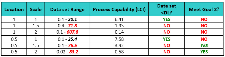
Table 2: Comparison of Simulated Data (Lognormal Distribution) and their Process Capability Results - As shown here, the lower confidence interval (LCI) is used as a "worst case" evaluation. Note: Since the threshold parameter was set at zero, there was no need to evaluate whether the data exceeded this boundary.

The simulations for both locations of 1 and 0.5 where the scale was largest (1.5 and 2) created data sets that had data points that exceeded the detection limits, so these were not acceptable. Using these parameters would result in process capabilities that are very low. The simulations where the scale was small (1) created data sets that had data points that did not exceed the detection limits, but the data values were only about ½ of the DL and using this parameter would artificially result in process capabilities that are very high and are also unacceptable. None of these simulations were found to be acceptable.

Figures 4, 5, 6, and 7 show the graphs generated from these data sets.

Figure 4: Process Capability for Simulated Lognormal Data with a Location of 1 and a Scale of 1.

Figure 5: Process Capability for Simulated Lognormal Data with a Location of 1 and a Scale of 2.

Figure 6: Process Capability for Simulated Lognormal Data with a Location of 0.5 and a Scale of 1.

Figure 7: Process Capability for Simulated Lognormal Data with a Location of 0.5 and a Scale of 2.

One way to guide the selection process is to explore what lognormal distributions look like at different parameter settings. Figure 8 shows a graph overlaying two lognormal distributions with different scale settings.

Figure 8: Lognormal Distribution Plot for Threshold Setting of 0 and Location Setting of 1 for Scale settings of 4 and 0.5. The distribution for the scale setting of 4 extends beyond the DL point of 50, while the distribution for the scale setting of 0.5 ends around 30.

The distribution with a scale setting of 4 extends beyond our chosen boundary of 50 and would not be appropriate for our analysis. The distribution with a scale setting of 0.5 extends only up to about 30 and could be appropriate for our analysis. Experimenting initially with distribution plots can save time for identifying the most appropriate parameter settings. Based on this exploration, a location of 0.5 with a scale setting of 1.25 was tried. These parameter settings yielded results that better met both goals 1 and 2. (Figure 9)

Figure 9: Process Capability for Threshold Setting of 0 and Location Setting of 0.5 and a Scale setting of 1.25.

Once again, the selection of the location and scale can be optimized. And, again, for HPLC data sets where all the data are less than the detection limits, excellent process capabilities would be expected. For these simulations and analyses, it is recommended that the locations and scales selected should generate data sets that are all below the detection limits and result in the lowest possible process capability scores as "worst case" estimates.

Subsequent to the publication of our article on partially censored data, an article by Donald Wheeler, Ph.D., on the use of the lognormal model was brought to the authors' attention.⁶ This article discusses how the lognormal should not necessarily be chosen based on skewness of data and that the majority of data in a lognormal distribution will be within two standard deviations regardless of the degree of skewness.⁷ The amount of data in the tails may actually be insignificant for many analyses. This observation may point us back to simply choosing the normal distribution as the model even when the data are found to be skewed.

Alternative Approaches

There are also other approaches that can be used to estimate the Cpu. When all the cleaning results are censored, the information available is not sufficient to estimate the distribution parameters (e.g., mean and standard deviation) and to infer about the capability of the cleaning process. However, if certain assumptions about the distributional characteristics can be made, then the following approaches can be used for the estimation of Cpu.

Approach Assuming A Normal Distribution

If it can be reasonably assumed or empirically demonstrated that the cleaning data is normally distributed, then using the method of Smith and Burns,⁸ a conservative value of Cpu can be estimated by maximizing the following function:

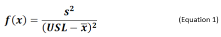
From the f(x) value, the Cpu value can be computed using the relationship below:

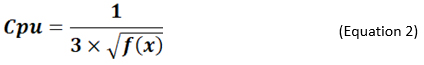
Where, x = {x1, x2, …, xn} is the data set of n observations and each observation xi less than the DL, x̄ is sample mean, and s the sample standard deviation.

The maximum value of f(x) can be obtained by generating a data set, consisting of only zeroes and the DL, and then computing the function in equation (1).

This approach can be easily performed using a spreadsheet.⁹

Approach Assuming A Normal Distribution And A Standard Deviation

This approach can be used where some prior information is available from previous cleaning validation studies or possibly from small-scale cleanability studies. For example, the type of sample distribution and the standard deviation (σ) of the sampling data may be known and available. Therefore, cleaning process capability could be analyzed if the mean (μ) could be calculated.

Assuming a normal distribution, and a given value of σ, a value for the mean (μ) can be easily solved using the relationship below:

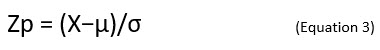
For example, for a sample size of 20 completely censored observations, the 95% lower bound for the observed proportion will be p_{95% lower} = 0.05^1/20 = 0.8609; that is, the true population value for the proportion of completely censored results lies in the range 0.86 to 1.00. The corresponding Zp will then be φ^-1(0.8609) = 1.0843 [note: this value can easily be obtained in Excel using the function =NORM.S.INV(0.8609)]. Assuming that the DL of the analytical method is 50 ppb, σ is 25, and the cleaning limit (USL) is 250 ppb, then the values of μ and Cpu are obtained as follows:

Solving Equation 3 for μ we get:

μ = X – Zp x σ

μ = DL – Zp x σ
μ = 50 - 1.0843 x 25 = 22.892

Cpu = (USL – μ)/ (3xσ)
Cpu = (250 – 22.892)/(3x25) = 3.028

When σ is unknown, the approximate value of the sample standard deviation can be estimated from the minimum and maximum values using the following equation of Wan et al.:¹⁰

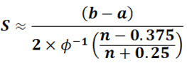
S is the sample standard deviation, b is the maximum value, a is the minimum value, n is the total number of observations, and φ^-1 is the inverse of the standard normal cumulative distribution function.

Setting b = DL=50 ppb, a = 0, the sample standard deviation for a sample size of 20 would be:

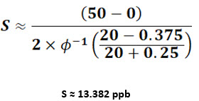
From the value of S, the mean and Cpu can be obtained as discussed earlier. For a data set of 20 observations and cleaning limit of 250 ppb, we will get the mean and Cpu values of 35.489 ppb and 5.343, respectively.

Figure 10 shows the overlaid probability distribution plot for the two data sets (with standard deviations of 25 and 13.382). From the comparison of the fitted probability curves, it appears that the data set with the standard deviation 25 ppb is left-truncated normally distributed with about 68% of the population expected to lie between zero and the DL. The Cpu based on a truncated normal distribution can be estimated using the method of Polansky et al.¹¹ On the other hand, for the data set with the standard deviation of 13.382 ppb, about 85% of the population is expected to lie between zero and the DL. Therefore, an approximate normal distribution can be reasonably assumed and Cpu can be computed using the equation Cpu = (Limit – μ)/ (3xσ).

Figure 10: Distribution Plot of Data sets with Standard Deviations of 25 ppb and 13.382 ppb.

Using the same approach as described above, the Cpu for lognormally distributed data can also be estimated.

Analytical Approach Using The Standard Addition Method.

Another approach that can be used that actually generates analytical data is the Standard Addition Method (SAM). The SAM has been used for many decades in analytical methods such as colorimetry, spectrography, and polarography.¹² The basic idea is that a sample containing a compound that is below the DL can have a standard amount of that compound added to the sample, bringing its concentration above the DL so it can be analyzed. The result is then the difference between the standard and the sample + the standard (Table 3).

Table 3: Analyzing a Sample using the Standard Addition Method - In this example, a sample is found to be less than the detection limit (75 ppb), so a known amount of the compound is added to the sample. This sample + standard amount is analyzed and compared to the standard itself. The difference between them is the actual amount of compound in the sample that could not be detected – in this example 23 ppb.

This approach can obtain actual values that can then be statistically evaluated for process capability. While this can be a significant amount of laboratory work, it would be a very useful way of determining the data distribution of the residues below the detection limit. Once this distribution is known, the process capabilities can be analyzed as shown above.

Note: This method is only valid when the method sensitivity (ability to measure the difference between the two values) and the method precision (measurement variability) are adequate to measure a true difference between a sample and the sample + added standard. If the true difference is small, simple method variability could be misinterpreted as a real result, leading to an incorrect process capability value.

Summary

As stated in the article on partially censored data, one of the goals of the ASTM E3106-18 Standard Guide¹³ was to provide a framework for implementing the FDA's Process Validation approach for cleaning processes. The calculation of process capability is therefore an important part of any science- and risk-based approach to cleaning validation.^14-16 This article has shown how process capability of cleaning processes can be estimated where 100 percent of the data are left-censored. Using techniques such as these will allow the risk associated with cleaning processes analyzed using HPLC to be measured where, in the past, it was believed that process capability could not be calculated. This is another important development, as the ability to calculate process capability for cleaning processes with 100 percent censored data allows the level of exposure to be estimated¹⁴ and the level of risk to be measured.¹⁵

The measurement of risk is very important since, in the science-, risk-, and statistics-based world of ASTM E3106, it is the level of risk that determines the level of effort, formality, and documentation necessary for cleaning validation.¹⁶ The science-, risk-, and statistics-based approaches of ASTM E3106 can provide companies with many operational efficiencies (e.g., visual inspection) while ensuring the safety of their patients.

Peer Review

The authors wish to thank Thomas Altman, Joel Bercu, Ph.D., Alfredo Canhoto, Ph.D., David Dolan, Ph.D., Parth Desai, Jayen Diyora, Andreas Flueckiger, M.D., Christophe Gamblin, Igor Gorsky, Jessica Graham, Ph.D., Crystal Hamelburg, Hongyang Li, Ajay Kumar Raghuwanshi, Siegfried Schmitt, Ph.D., and Osamu Shirokizawa for reviewing this article and for providing insightful comments and helpful suggestions.

References

1. Walsh, Andrew, Miquel Romero Obon and Ovais Mohammad "Calculating Process Capability Of Cleaning Processes With Partially Censored Data" Pharmaceutical Online, May 2022.
2. Walsh, Andrew, Miquel Romero Obon and Ovais Mohammad " Calculating Process Capability Of Cleaning Processes: Analysis Of Total Organic Carbon (TOC) Data" Pharmaceutical Online, January 2022.
3. Denny, M. and Gaines, S. [2000]: "Chance in Biology: Using Probability to Explore Nature", Princeton: Princeton University Press.
4. Walsh, Andrew, Miquel Romero Obon and Ovais Mohammad "Calculating Process Capability of Cleaning Processes: A Primer" Pharmaceutical Online November 2021.
5. Limpert, Eckhard, Werner A. Stahel, and Markus Abbt "Log-normal Distributions across the Sciences: Keys and Clues" BioScience. May 2001 / Vol. 51 No. 5.
6. Email correspondence from Stan Alekman titled "The Lognormal" dated Tue 5/24/2022 6:51PM.
7. Wheeler, Donald, Ph.D. "Properties of Probability Models, Part 3: What they forgot to tell you about the lognormals" Quality Digest Daily, October 5, 2015.
8. Smith, D.E., & Burns, K.C. (1998). "Estimating percentiles from composite environmental samples when all observations are nondetectable". Environmental and Ecological Statistics, 5, 227-243.
9. Completely Censored Data Cpu Spreadsheet October 2022 DOI: 10.13140/RG.2.2.31486.25926 https://www.researchgate.net/publication/364341324_Completely_Censored_Data_Cpu
10. Wan, X., Wang, W., Liu, J., & Tong, T. (2014). “Estimating the sample mean and standard deviation from the sample size, median, range and/or interquartile range”. BMC medical research methodology, 14, 135. https://doi.org/10.1186/1471-2288-14-135.
11. Polansky, A. M., Chou, Y. M., & Mason, R. L. (1998). “Estimating process capability indices for a truncated distribution”. Quality Engineering, 11(2), 257-265.
12. Burns, D. Thorburn and Michael J. Walker "Origins of the method of standard additions and of the use of an internal standard in quantitative instrumental chemical analyses" Analytical and Bioanalytical Chemistry (2019) 411:2749–2753 https://doi.org/10.1007/s00216-019-01754-w
13. American Society for Testing and Materials (ASTM) E3106-18 "Standard Guide for Science-Based and Risk-Based Cleaning Process Development and Validation" www.astm.org.
14. Walsh, Andrew, Ester Lovsin Barle, David G. Dolan, Andreas Flueckiger, Igor Gorsky, Robert Kowal, Mohammad Ovais, Osamu Shirokizawa, and Kelly Waldron. "A Process Capability-Derived Scale For Assessing Product Cross-Contamination Risk In Shared Facilities" Pharmaceutical Online, August 2017.
15. Walsh, Andrew, Thomas Altmann, Alfredo Canhoto, Ester Lovsin Barle, David G. Dolan, Andreas Flueckiger, Igor Gorsky, Jessica Graham, Ph.D., Robert Kowal, Mariann Neverovitch, Mohammad Ovais, Osamu Shirokizawa and Kelly Waldron "Measuring Risk in Cleaning: Cleaning FMEA and the Cleaning Risk Dashboard" Pharmaceutical Online, April 2018
16. Walsh, Andrew, Thomas Altmann, Ralph Basile, Joel Bercu, Ph.D., Alfredo Canhoto, Ph.D., David G. Dolan Ph.D., Pernille Damkjaer, Andreas Flueckiger, M.D., Igor Gorsky, Jessica Graham, Ph.D., Ester Lovsin Barle, Ph.D., Ovais Mohammad, Mariann Neverovitch, Siegfried Schmitt, Ph.D., and Osamu Shirokizawa, Osamu Shirokizawa and Kelly Waldron, "The Shirokizawa Matrix: Determining the Level of Effort, Formality and Documentation in Cleaning Validation", Pharmaceutical Online, December 2019.