
How Much Measurement Error is Too Much? Part II: Acceptance Decisions in Real Processes
By R.K. Henderson, DuPont Photomasks Inc.
In the most general terms, this paper provides a theoretical basis for evaluating the relative magnitude of measurement process error and using measurement data to determine whether or not a specific product characteristic meets a supplied specification. Electronics-related industries have generally agreed that measurement error spread should be no larger than 10% of the allowable product specification window. Process industries, such as chemicals and textiles, have operated for years without meeting this 10% criterion. Part I of this paper borrowed a framework from the process industries for evaluating the impact of measurement error variation in terms of both customer and supplier risk (non-conformance and yield loss). Part II applies the resulting model to realistic process and measurement variations.
Perfect measurement techniques do not exist, and measurement error variance is never equal to zero. Once the measurement error variance is recognized to be greater than zero, the product acceptance decision becomes a bivariate problem. The two variables of concern are the Actual Product Value and the Observed Data Value. Using the assumptions of Part I of this work, it follows that these two variables have a joint bivariate normal probability distribution.
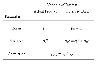
A bivariate normal distribution is defined by five parameters—the mean and variance values of each of the variables, and the correlation between them. Table 1 displays the values of the bivariate normal parameters for the variables of interest.
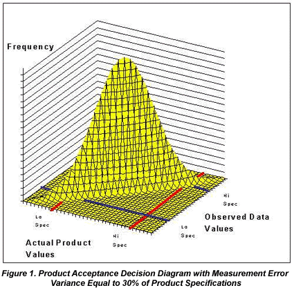
Most often, processes are somewhere between these two extremes. With any magnitude of measurement error (any correlation less than one), the probability of an occurrence in an error area is non-zero. Figure 1 shows a bivariate normal distribution for the case where measurement error variation is equal to 30% of the product specification window. There is some frequency of occurrences in the error areas.
Of course, the vast majority of the occurrences still fall in the correct areas. In order to obtain the probability of making an error in the decision process, it is necessary to determine the volume under the frequency curve in the area(s) of interest. These volumes can be obtained with relatively simple numerical integration using the approach outlined by Owen. Figure 2 shows the corresponding area probabilities obtained from the model depicted in Figure 1.
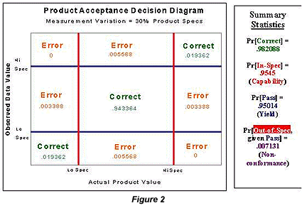
The sum of the nine area probabilities is equal to one. The sum of the three lower left to upper right diagonal areas is equal to the probability of a correct decision; this probability subtracted from one gives the probability of an incorrect decision.
There are several other probabilities of interest in this problem. The sum of the probabilities along the middle column represents the true production process capability. The sum of the probabilities across the middle row represents represents the process yield with application of the effective decision rule: to accept the product if the observed data value meets the specifications. Most often when capability is expressed as probability of meeting (or not meeting) specifications, a value similar to the process yield is quoted. When measurement error is present, traditional estimates of process capability include it and, as a result, will underestimate the true capability of the production process.
Another interesting value is the probability in the center area divided by the yield. This value represents the probability that product passing the decision rule and potentially shipped to a customer actually meets the requested specifications. One minus this value provides the probability that non-conforming product will be passed for shipment. Either of these values could be used to describe the capability of the process with the added step of applying the pass/reject decision rule to the measurement data obtained to evaluate the product characteristic of interest.
The specific situation depicted in Figures 1 and 2 pre-supposes a production process capability index, Cpk = Cp = .667. In other words, the production process would be expected to routinely produce product meeting the specifications only a little over 95% of the time. This process with the added product pass/fail decision would be expected to send on product meeting the specifications over 99% of the time. The cost of this "improvement" is the approximate 5% yield loss, of which only ~80% (or ~4% in total) is truly outside specifications.
The framework discussed above allows evaluation of an array of production process and measurement process variation combinations for their respective potential to provide product that meets specifications. Figure 3 displays non-conformance values for such an array of processes. The respective variation percentages are relative to the width of the specifications. Recall that non-conformance is the frequency with which product not meeting specifications passes the decision process.
Figure 3 suggests that the magnitude of measurement error variation (defined as 3sM) has only a minor effect on non-conformance. Changes in non-conformance are almost totally determined by the relative magnitude of the production process variation. At virtually any specific value of product variation, the non-conformance remains almost constant across the corresponding range of measurement variation values. Thus, Figure 3 suggests that the magnitude of measurement error variation is of little to no importance. This is indeed a valid conclusion with respect to the potential of a process and a corresponding data-driven decision rule to provide product meeting specifications to a customer.
There appear to be some marginal gains when the measurement error variation is less than 20% of the specification window. However, these gains only hold practical significance for processes that are already having substantial difficulty meeting the specifications (Cp < .75). The real message of Figure 3 is that there is no substitute for a good production process.
Unfortunately, Figure 3 fails to demonstrate the cost to the supplier to provide these very small non-conformance values. Figure 4 displays the respective yield values for the same array of variation scenarios shown in Figure 3. In this figure, the effect of large measurement error is more pronounced, as there actually is some meaningful change in yield vertically across the variation space.
Figure 4 suggests that measurement error variation does have a significant effect with respect to the yield of the process with the pass/fail decision applied. But again, the real message of Figure 4 is that there is still no substitute for a good process. For a Cp=2 production process, yield will still be greater than 99% even when the measurement process variation is 100% of the width of the product specifications. Alternatively, for a Cp=.5 production process, yield is below 87% even when the 10% measurement variation criterion is satisfied.
Conclusions
How much measurement error is too much? The default answer, "any amount is too much," is not realistic. As a practical matter, a 10% criterion has been widely applied. The framework discussed in this paper suggests that the 10% criterion is, in many cases, probably much more stringent than necessary. For a Cp=1 production process with an appropriate pass/fail decision process applied to data acquired to describe it, the non-conforming product passed for potential shipment to a customer will remain very close to 0.1% regardless of the magnitude of the measurement error variation. Yield for such a process will remain greater than 99% for measurement error variation as large as 60% of the specification window. Ultimately, the tolerable amount of measurement error is largely dependent on the capability of the actual production process involved.
The approach discussed in this paper provides a means for evaluating specific situations in order to provide a potentially more reasonable estimate of tolerable measurement error variation. Admittedly, the model discussed is in its simplest form. It can be, and has been, extended to more complicated, yet more realistic variance component models for both of the processes involved. A more realistic variance component model supports evaluation of the impact of various sampling plans. More elaborate variance component structures and/or manipulation of related sampling plans provide no meaningful changes to Figures 3 and 4 above, or any relevant conclusions that might be drawn from them.
The basic approach here can also evaluate the potential impact of operating either, or both the production process and measurement process away from their respective target values. Such biases can dramatically alter both Figures 3 and 4. Non-conformance and yield are much more dramatically impacted by off-target operation than by increases in production or measurement process variation. Still, with the application of effective process control schemes, there is negligible difference in non-conformance and yield for measurement error variation from the accepted 10% level up to 30 to 40%.
Finally, and perhaps most importantly, this paper is not intended to encourage sloppiness in managing measurement processes. Effective control of measurement processes is critical to successfully supplying customers, and effective control of any process is essentially bounded by the process precision. While a measurement error variation of 10% would always be desirable over some larger value, operations can remain viable even though in violation of the 10% criterion. This work is primarily intended to show that when best possible practices still fail to satisfy the 10% criterion, there is no need for paranoia to rule subsequent discussions, or more importantly, continued process operations.
For more information: R.K. Henderson, DuPont Photomasks Inc., Reticle Technology Center, Round Rock, TX 78664. Tel: 512-310-6409. Email: robert.henderson@photomask.com.